Principal Component Analysis
From EosPedia
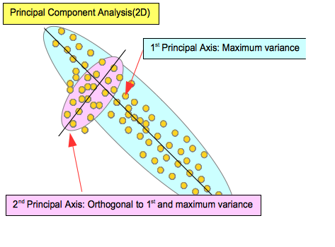
Principal Component Analysis is the method that calculates from vector data set which has elements of Multivariate to the axis (principal axis) which has maximum variance when each vector data is projected into that axis on Multivariate Space, and calculates the axis sequentially that is orthogonal(no correlation) to it and has largest variance.
Execution example of PCA
PCA of each image
Classify multiple images by using mrcImagePCA mainly.
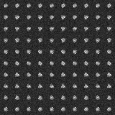
Input file's image
rotate the image at 10 pattern (vertical), and add noise at 10 pattern (Horizontal). (Sum 100)
First, calculates principal axis by using mrcImagePCA.
NO2_ROI_LIST's data
Target-1-0-0-0.nroi
Target-1-0-0-1.nroi
Target-1-0-0-2.nroi
Target-1-0-0-3.nroi
Target-1-0-0-4.nroi
Target-1-0-0-5.nroi
Target-1-0-0-6.nroi
Target-1-0-0-7.nroi
Target-1-0-0-8.nroi
Target-1-0-0-9.nroi
Target-37-0-0-0.nroi
Target-37-0-0-1.nroi

...

Target-289-0-0-8.nroi
Target-289-0-0-9.nroi
Target-325-0-0-0.nroi
Target-325-0-0-1.nroi
Target-325-0-0-2.nroi
Target-325-0-0-3.nroi
Target-325-0-0-4.nroi
Target-325-0-0-5.nroi
Target-325-0-0-6.nroi
Target-325-0-0-7.nroi
Target-325-0-0-8.nroi
Target-325-0-0-9.nroi
TEST_PCA_LIST's data
Target-1-0-0-0.tpca
Target-1-0-0-1.tpca
Target-1-0-0-2.tpca
Target-1-0-0-3.tpca
Target-1-0-0-4.tpca
Target-1-0-0-5.tpca
Target-1-0-0-6.tpca
Target-1-0-0-7.tpca
Target-1-0-0-8.tpca
Target-1-0-0-9.tpca
Target-37-0-0-0.tpca
Target-37-0-0-1.tpca

...

Target-289-0-0-8.tpca
Target-289-0-0-9.tpca
Target-325-0-0-0.tpca
Target-325-0-0-1.tpca
Target-325-0-0-2.tpca
Target-325-0-0-3.tpca
Target-325-0-0-4.tpca
Target-325-0-0-5.tpca
Target-325-0-0-6.tpca
Target-325-0-0-7.tpca
Target-325-0-0-8.tpca
Target-325-0-0-9.tpca
Command
mrcImagePCA -i NO2_ROI_LIST -o TEST_PCA_LIST -NX 39 -NY 39 -numE 20 -O EIGEN_INFO -E eigen -EPS 100;
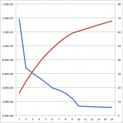
Check the eigenvalues after command run.
EIGEN_INFO's data
   0   485  13783745.48  16.25
   1   600  6874158.21  24.36
   2   997  6040647.42  31.48
   3   529  5425460.64  37.88
   4   834  4720681.32  43.45
   5   879  3932086.98  48.08
   6   842  3632776.78  52.37
   7   645  3182620.81  56.12
   8   566  2449230.98  59.01
   9  1116  1328891.76  60.57
  10  1031  1287023.24  62.09
  11   579  1257054.49  63.57
  12  1080  1214056.15  65.01
  13   856  1161105.65  66.38
  14   934  1144996.99  67.73

...
Data are arranged in the order of height of the eigenvalues (3rd columns). See the figure below. In this case, Eigenvalues of up to the 8th component is higher than others. You can see that it can be explained up to 60% dispersion.
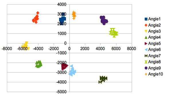
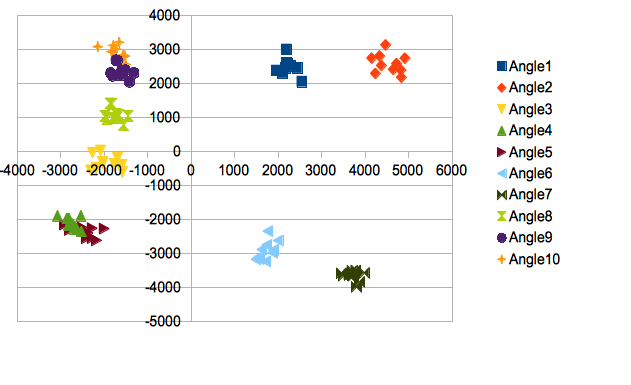
Look about the scatter plot at 1st ~ 3rd component.
The file specified at mrcImagePCA's option -o is stored the vector elements of each image in the order of height of the eigenvalues. Thus, by using upper level of this data, you can see which group the image is belong. In addition, by using mrcImageMakeDump, mrcImage's data can be output as ASCII.
	-1002.110000	1962.390000	2375.080000	3780.900000	1531.830000	-3511.960000	-524.329000	1190.540000	-1106.170000	337.342000
	-1111.780000	2439.510000	2452.540000	3826.020000	1630.650000	-3519.130000	-457.767000	1531.510000	-316.514000	-2399.750000
	-844.584000	2207.500000	2577.200000	3895.480000	1722.810000	-3401.740000	-573.914000	961.414000	-1120.780000	75.002400
	-897.296000	2107.620000	2308.710000	3974.960000	1590.460000	-3559.020000	-836.757000	1690.460000	-332.499000	46.332400
	-639.501000	2286.200000	2513.990000	3868.320000	1741.350000	-3316.310000	-553.213000	1443.870000	-1044.260000	560.677000
	-1015.980000	2549.020000	2049.920000	3854.560000	1503.460000	-3118.820000	-919.956000	1212.420000	-792.175000	1047.500000
	-892.673000	2168.280000	2455.920000	3951.430000	1400.510000	-3498.790000	-528.413000	1509.180000	-1141.580000	10.826800
	-799.775000	2190.870000	2994.040000	3730.140000	1208.160000	-3002.190000	-538.733000	800.946000	-1115.250000	380.240000
	-1061.460000	2100.710000	2348.670000	3881.800000	1573.210000	-3440.970000	-606.476000	1363.520000	-649.180000	422.532000
	-782.003000	2198.650000	2594.880000	3976.130000	1891.720000	-3371.260000	-531.849000	1410.830000	-957.755000	148.813000
	-4295.390000	4650.010000	2406.060000	-2699.870000	1602.340000	2108.780000	1198.180000	-963.790000	565.743000	256.211000
	-4371.810000	4724.700000	2581.440000	-2274.290000	1625.690000	1392.540000	1677.500000	-492.734000	770.713000	-2612.010000

...

	533.205000	-1655.000000	3206.460000	1451.350000	-4268.840000	-120.817000	900.958000	-2478.230000	428.414000	361.083000
	667.314000	-1569.670000	2828.330000	1229.300000	-4102.610000	-108.603000	1067.760000	-2409.760000	875.312000	-147.388000
	703.368000	-1789.180000	3114.700000	1694.560000	-4408.100000	-286.116000	1112.690000	-2717.040000	595.316000	-136.777000
	546.967000	-2147.200000	3076.260000	1691.570000	-4386.750000	-567.557000	963.625000	-2624.400000	913.221000	-49.355200
	567.210000	-1505.020000	2555.640000	1290.990000	-4242.580000	-407.482000	1022.360000	-2779.230000	636.427000	308.664000
	727.232000	-1522.510000	2804.310000	1861.250000	-4377.870000	-163.006000	1417.020000	-2410.950000	776.618000	186.569000
	538.177000	-1556.390000	2774.820000	1342.150000	-4350.580000	-378.349000	1186.870000	-2627.670000	619.576000	60.747200
	466.937000	-1725.230000	3004.230000	1525.800000	-4514.230000	-370.642000	1165.460000	-2520.760000	654.709000	54.430900
Incidentally, by using Input fileに対してThis Makefile and running at the following commands, you can execute the method of up to here.
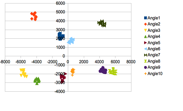
Collect 10 rows of this file as 1 angle's data, and display the scatter plot whose axis is as each column.
the scatter plot by 1st(Vertical) and 2nd(Horizontal) |
the scatter plot by 1st(Vertical) and 3rd(Horizontal) |
the scatter plot by 2nd(Vertical) and 3rd(Horizontal) |
Classify the images based on the scatter plot. If its pattern is above 10, it means that on 3D they can be almost classified.
